

 EnglishEN
 ItalianoIT
 DeutschDE
 PortuguêsPT
 FrançaisFR
 РусскийRU
MAF scaling guide workflows should start from the exact ECU strategy, sensor type, intake geometry and logging capability rather than from one universal multiplier or AFR target. A geometric area ratio can be a useful starting estimate after a housing change, but final calibration must be based on reliable logs, the ECU’s actual load model and platform-specific fuel-control behavior.
- Closed-loop validation: review fuel trims only in operating areas where the ECU is actually using closed-loop correction.
- High-load validation: compare commanded and measured lambda with a suitable wideband or validated OEM lambda strategy.
- Curve quality: keep the transfer function smooth and physically plausible without forcing a universal shape.
- Cross-checks: use MAP/Speed Density or other load-model data only when that reference model is itself validated.
Common validation methods include closed-loop trim analysis, high-load lambda logging and comparison with a validated Speed Density or modeled-airflow reference where supported. Not every ECU or project requires all three methods.
MAF Scaling Guide: Key Takeaways
A professional MAF scaling guide uses geometry only as a starting estimate, then validates the ECU’s actual airflow model with trustworthy logs and platform-specific lambda/fuel-control behavior.
| Punto | Detalles |
|---|---|
| Geometry is only a starting estimate | Housing-area ratio can help after a simple diameter change, but it is not a finished calibration. |
| Fuel trims are not MAF-only data | Leaks, injectors, pressure, lambda sensors and compensations can move trims. |
| High-load lambda targets are platform-specific | Do not use one universal AFR target for every gasoline engine. |
| Speed Density is not an absolute reference | Use it only when MAP/IAT and the VE/load model are already validated. |
| Change only what the logs support | Avoid extrapolating large corrections into untested voltage or frequency regions. |
| TuningBot can support outsourced calibration | The workshop still provides accurate hardware data, logs and final validation. |
MAF Scaling Guide: Tools, Data and Conditions
Reliable MAF calibration requires trustworthy logging and a mechanically sound intake system. The exact sensors and channels depend on the ECU and vehicle.
Essential hardware:
- A suitable lambda measurement method where the OEM sensor/logging strategy is insufficient for the calibration task.
- Logging capable of capturing the MAF signal plus the load, lambda and correction channels relevant to the ECU.
- Laptop with your ECU tuning software installed and a working communication interface
- A safe, legal test area for power runs; a fire extinguisher in the vehicle if doing dyno or road pulls
- A known-good fuel source: same octane, same station, consistent across all logging sessions
Critical logging channels to enable:
- MAF voltage (V) and MAF mass flow (g/s or kg/hr)
- Commanded AFR and wideband AFR
- LTFT and STFT (both banks if applicable)
- RPM, MAP (manifold absolute pressure), IAT (intake air temperature), throttle position
- Engine load (calculated or normalized), battery voltage
Electrical stability matters during both logging and ECU programming, but sensor-supply behavior should be diagnosed from actual voltage data rather than assumed from battery condition alone.
Environmental checklist:
- Document ambient and intake temperatures so changes in conditions can be separated from calibration errors.
- Use the same fuel octane across all calibration sessions
- Confirm no active DTCs before logging; a pending misfire or O2 heater fault corrupts trim data
- Secure the vehicle on the dyno or confirm a safe road stretch before open-loop pulls
Consejo profesional: Warm the engine fully before collecting any baseline log. A cold engine runs open-loop enrichment, which masks the true LTFT behavior you need to see. Let coolant temperature stabilize and take at least two warm-up laps before recording data you intend to use.
Hardware changes like upgraded intakes also affect the broader ECU calibration, not just the MAF table. Reviewing stage 2 hardware upgrade requirements before logging gives you a clearer picture of what else may need attention.
How does MAF sensor output actually control fuel delivery?
Many ECUs use MAF data as an important input to load and fuel calculations, but the exact role varies by architecture and may be cross-checked against MAP, throttle, lambda and modeled airflow.
Signal types and ECU interpretation:
- Hot-wire MAF sensors output an analog voltage (typically 0–5 V) that rises with airflow. The ECU holds a lookup table mapping each voltage to a g/s value.
- Frequency-output MAF sensors (common on some GM and Bosch applications) output a variable-frequency signal; the ECU maps frequency to g/s through a similar transfer table.
- Vane-meter MAF sensors (older designs, still found on some Japanese platforms) use a mechanical flap and potentiometer; they are more sensitive to backflow and turbulence than hot-wire designs.
Changing housing diameter, sensor position, upstream bends or filter geometry can alter the relationship between sensor output and total airflow. Whether rescaling is required and by how much depends on the actual sensor and ECU strategy.
As Mishimoto’s engineering analysis notes, even a modest increase in housing diameter can produce a meaningful shift in sensor resolution at idle, where the sensor element operates near the bottom of its voltage range and small geometry changes have disproportionate effects.
Fuel trims can reveal systematic air-model or fueling errors in closed-loop operation, but they also reflect injector characterization, fuel pressure, leaks, sensor bias and other corrections. They should not be attributed to MAF scaling alone.
How do you calculate the initial coarse multiplier from housing dimensions?
Cross-sectional area can provide a first estimate when only the housing diameter changes and the sensor arrangement remains comparable. It is not guaranteed to produce a safe starting point on every intake design.

The formula:
Area = π × r²
where r = inner radius of the MAF housing in millimeters (or inches, as long as you are consistent).
Multiplier = Area_new ÷ Area_old
Worked example: 65 mm stock housing → 80 mm aftermarket pipe
- Area_old = π × (32.5)² = π × 1,056.25 = 3,318.3 mm²
- Area_new = π × (40.0)² = π × 1,600.0 = 5,026.5 mm²
- Multiplier = 5,026.5 ÷ 3,318.3 = 1.515, or approximately +51.5%
Do not apply the geometric multiplier blindly across the entire transfer curve. Use it only as a coarse estimate where the hardware change justifies it, then verify actual sensor behavior before extending the correction into unlogged regions.
Starting multiplier for a 65 mm to 80 mm housing change: approximately ×1.515 on all g/s values. This is a geometric estimate only; flow profile, sensor placement, and turbulence from bends will shift the final curve away from this starting point in every real-world installation.
Limitations of area-only scaling:
- The formula assumes uniform, laminar flow across the sensor element, which is rarely true in a real intake
- Sensor position relative to the housing centerline affects local velocity; off-center elements read differently than centered ones
- Bends, couplers, and filter housings upstream of the sensor create turbulence that changes the effective flow profile
- The area multiplier scales the whole table by a single factor; the actual correction needed often varies across the voltage range
HP Academy’s MAF rescaling course material confirms this directly: area math produces a useful coarse starting point, but the final curve almost always requires reshaping because housing geometry and sensor placement change turbulence and local flow velocity in ways the formula cannot predict.
How do you use closed-loop fuel trims to refine MAF scaling at idle and cruise?
Closed-loop operation is useful for low- and part-load refinement when the ECU is actively using lambda feedback. Confirm the relevant operating state before interpreting trims.
- Collect stable closed-loop data across the relevant idle, cruise and light-load regions while avoiding obvious transients.
- Analyze trims against MAF signal and operating state, then rule out leaks, injector scaling and pressure errors before changing the MAF table.
- Use trim data as a directional correction signal; the exact mathematical update depends on ECU strategy and how the transfer table is defined.
- Re-log under comparable conditions and confirm that the correction improved the relevant region without creating errors elsewhere.
- Use platform-specific trim expectations and repeatability rather than a universal pass/fail percentage.
- Verify injector scaling and compensations. LTFT reflects multiple ECU corrections simultaneously. If trims behave unexpectedly after MAF adjustments, confirm injector scaling and temperature compensation tables are correct before assuming the MAF table is the sole source of error.
Consejo profesional: Average at least three separate closed-loop logs taken on different days and at similar ambient temperatures before committing to a correction. A single log can contain outliers from transient conditions, traffic stops, or brief sensor anomalies. Averaged data produces a more accurate picture of the true trim offset at each MAF voltage point.
How do you rescale the MAF table using open-loop wideband AFR runs?
At high load, some ECUs reduce or change closed-loop authority while others retain wideband feedback. Use the platform’s actual lambda-control strategy rather than assuming all high-load operation is open-loop.
- Use the lambda target appropriate to the engine, fuel, boost and OEM protection strategy; do not apply a universal gasoline AFR target.
- Do not flatten unrelated fuel tables simply to isolate MAF error unless the platform-specific calibration method explicitly calls for it.
- Collect high-load data only in a safe, controlled environment and log the channels required by the platform.
- Compare commanded and measured lambda together with fuel pressure, trims, injector control and MAF signal before assigning the error to MAF scaling.
- Apply corrections at logged voltage points. Edit only the voltage points you have actual logged data for. The ECU interpolates between set points, so a smooth, well-spaced set of corrections produces a clean curve without abrupt transitions.
- Repeat validation until the model is stable and matches the platform-specific target across the tested region.
Sample open-loop log structure:
Consejo profesional: After applying corrections, smooth the MAF curve using your software’s smoothing function before the next pull. A jagged curve with sharp steps between voltage points creates AFR spikes and can trigger knock events at the transition points. The curve should rise steadily with no reversals or flat spots.
MoviChip’s MAF calibration documentation describes this same point-by-point interpolation approach, recommending adjustments in voltage steps across the 0–5 V range and targeting fuel trims near ±5% as the calibration goal.
How does Speed Density help you verify or replace MAF scaling?
Speed Density estimates cylinder air charge from pressure, temperature, displacement and a calibrated VE or load model. It can be a useful reference only when those inputs and the reference model are already trustworthy.
- Confirm MAP and IAT plausibility and stability before using a Speed Density reference.
- Enable SD or hybrid mode in your tuning software. On EcuTek platforms with RaceROM, this is a dedicated parameter. The ECU begins calculating SD-based mass airflow in parallel with the MAF sensor output.
- Compare modeled and measured airflow only where both signals are known to be valid.
- Do not force the MAF curve to match an unvalidated SD estimate; investigate the cause of disagreement first.
- Re-check the final calibration using the ECU’s actual low-load and high-load control strategies.
EcuTek RaceROM provides platform-specific Speed Density tools that can assist MAF comparison on supported applications. That workflow should not be generalized to unrelated ECUs.
When SD is the better primary strategy:
- The MAF sensor has been relocated far from its factory position
- Intake changes are so significant that the MAF voltage output is erratic or non-monotonic
- The build has outgrown the stock MAF’s measurement range at high load
As HP Academy’s MAF vs. SD analysis notes, MAF suits bolt-on modifications well, while SD gives more headroom for extreme builds where the stock sensor is a limiting factor.
Consejo profesional: Use SD as a cross-check only after you have confirmed MAP sensor stability and that your VE table is accurate for your specific platform. An SD reference built on a VE table that was never validated for your camshaft or compression ratio will mislead you as reliably as a poorly scaled MAF table.
A worked example: before-and-after logs showing iterative MAF correction
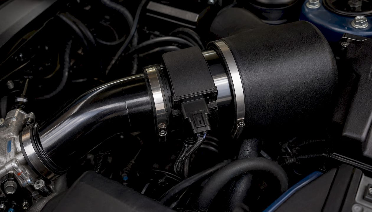
The following BRZ example illustrates one possible iterative workflow. Its numbers are examples, not universal calibration targets.
Baseline condition (no multiplier applied):
In this illustrative example, the logged trims and measured lambda indicate a large airflow-model mismatch after the housing change.
Round 1: area multiplier applied
- Area_old (65 mm): π × (32.5)² = 3,318.3 mm²
- Area_new (75 mm): π × (37.5)² = 4,417.9 mm²
- Multiplier: 4,417.9 ÷ 3,318.3 = 1.331
All g/s values scaled by ×1.331.
Round 2: closed-loop refinement
Round 3: open-loop verification
Full-throttle pull from 2,500 RPM to 7,000 RPM. Wideband AFR at 4.0 V: 12.1:1. At 4.5 V: 11.9:1. Both within the 11.8–12.2:1 target band. No further corrections required at those voltage points.
Three-round iteration result: LTFT from +15% baseline to +1–2% at idle/cruise; open-loop AFR from 13.1:1 to 12.1:1 at peak load. This is the expected progression when area math, closed-loop refinement, and open-loop verification are applied in sequence.
For best practices on capturing and organizing log data across multiple sessions, structured data-handling workflows like those described in CMM data import practices offer a useful framework for maintaining version-controlled calibration records.
Which hardware and software tools do US tuners need for MAF calibration?
For a MAF scaling guide, tool choice depends on vehicle coverage, required channels, sensor integration and calibration software. No single toolset is mandatory for professional MAF work.
Wideband O2 kits:
- AEM X-Series (part 30-0300) and Innovate Motorsports LC-2 are the two most widely used standalone widebands in US shops. Both use the Bosch LSU 4.9 sensor and output 0–5 V analog for datalogger integration.
- For EcuTek-based platforms, the EcuTek wideband module integrates directly into the RaceROM logging environment, eliminating the need for a separate analog input.
Dataloggers and scan tools:
- EcuTek ProECU handles logging, table editing, and SD mode on Subaru, Toyota GR, and other supported platforms. It captures all required channels natively.
- For platforms outside EcuTek’s coverage, HP Tuners MPVI3 and EFI Live cover a wide range of GM, Ford, Chrysler, and other US-market ECUs with full MAF table editing capability.
- Tactrix Openport 2.0 is a cost-effective logging interface for Subaru and Mitsubishi platforms running open-source or EcuTek software.
EcuTek and RaceROM specifically:
EcuTek ProECU and RaceROM provide integrated logging and calibration functions on supported platforms. Other ECU families may require different software and interfaces.
Buying and renting guidance:
- A quality wideband kit ($200–$350) is a permanent workshop investment; do not rent this.
- High-end dyno time is the more practical rental: most US dyno shops charge per session and provide their own load cell and logging infrastructure.
- If you tune a single platform infrequently, renting EcuTek ProECU licenses per vehicle is more cost-effective than a full annual subscription.
Accuracy criteria to prioritize:
- Wideband sensor response time under 250 ms for accurate transient logging
- MAF voltage resolution of at least 0.01 V in your logger to distinguish adjacent table points
- Software that supports direct g/s table editing, not just multiplier-based scaling, for precise point-by-point correction
What are the most common MAF scaling mistakes and how do you fix them?
MAF-scaling problems often come from poor data quality, intake leaks, sensor contamination, injector/fuel-pressure errors or over-aggressive table edits.
- Relying on insufficient data: use enough repeatable logs to separate real calibration error from transient noise.
- Ignoring learned adaptations: understand the ECU’s adaptation strategy before clearing or interpreting learned values.
- Over-scaling: large unsupported corrections can distort calculated load and fueling; change only regions supported by reliable data.
- MAF sensor contamination. Oil from a poorly sealed catch can or an over-oiled cotton filter element coats the hot-wire element and shifts the transfer curve unpredictably. If LTFT drifts positive over weeks without hardware changes, inspect and clean the sensor element with MAF-safe cleaner before recalibrating.
- Intake leaks: unmetered or lost air can invalidate both MAF and fuel-trim conclusions; pressure/smoke-test the intake where appropriate.
- MAF voltage noise from grounding issues. A noisy MAF voltage signal (visible as rapid oscillation in the log at steady throttle) indicates a grounding or shielding problem. Check the MAF sensor ground path back to the ECU chassis ground and inspect the wiring harness for chafing near exhaust components.
- Interpolation artifacts from uneven point spacing. If you correct only a few voltage points and leave large gaps, the ECU’s linear interpolation between those points can create a step in the effective g/s curve. Correct at evenly spaced voltage intervals and smooth the curve after each editing session.
Common fault patterns from poor tuning covers how MAF scaling errors propagate into ignition timing and load calculations, which is useful context when diagnosing symptoms that go beyond fuel trims alone.
Final verification checklist before declaring the MAF rescale complete
A MAF scaling guide final validation should cover the operating regions actually used by the vehicle and should be repeated when hardware or environmental conditions change materially.
- Review STFT/LTFT against the platform’s normal range and repeatability; do not use one universal ±5% threshold for every ECU.
- Use the lambda target appropriate to the engine, fuel, boost and OEM protection strategy; do not apply a universal gasoline AFR target.
- MAF curve shape: The g/s vs. voltage curve rises monotonically with no reversals, flat spots, or sharp steps. Plot it visually in your software before finalizing.
- No new DTCs: Clear codes after the final calibration and drive a full OBD-II readiness cycle. Any new MAF-related, O2, or load-calculation codes indicate an unresolved issue.
- MAP/IAT plausibility: signals are stable enough to support any modeled-airflow cross-check.
- Environmental robustness: verify that normal temperature changes do not create abnormal trim or load-model behavior.
- Adaptation follow-up: re-check learned trims after sufficient normal operation for the specific ECU to update its adaptations.
What professional tuners actually do differently when scaling a MAF
Professional calibration depends on disciplined logging, version control, repeatable testing and willingness to revise the model when the data disagrees with the initial estimate.
Professional tuners treat every intake iteration as a separate calibration event. When a customer returns with a different filter, a relocated sensor, or a revised intake pipe, the calibration file is versioned and the previous log set is retained. That history makes the next iteration faster because the tuner can see exactly where the previous curve diverged and predict where the new hardware will shift it.
Geometric scaling is only a hypothesis. Logged behavior should determine the final transfer curve.
Use enough repeatable data to distinguish a pattern from transient noise. There is no universal requirement for exactly three sessions.
Re-verify MAF calibration after meaningful intake, sensor or fuel-system changes. Ordinary ambient-temperature variation alone does not automatically require rescaling if the ECU compensations are working correctly.
When to Outsource MAF Calibration
When a workshop does not have reliable definitions, logging capability or enough platform experience, outsourcing the ECU file can reduce development time.
Before ordering, check Cobertura del servicio ECU, repasa la Lista de Precios Pública y busca las disponibles Servicios ECU.
El archivo original puede enviarse a través de Reprograma tu archivo without prepaid credits.
For related internal references, see Medición y modelización de la masa de aire y las Guía de ajuste de mapas de combustible.
The workshop remains responsible for accurate hardware information, vehicle diagnosis, programming and final validation.
Sources and Further Reading
- EcuTek RaceROM Speed Density — external platform-specific MAF/SD reference.
- Mishimoto MAF vs Speed Density — external engineering overview.
- HP Academy MAF Rescaling — external training reference.
- EcuTek Intake/MAF Rescaling — external platform-specific intake scaling reference.
- TuningBot Air Mass Measurement and Modeling — internal ECU airflow-model reference.
- TuningBot Fuel Map Tuning Guide — internal fuel and airflow calibration reference.
PREGUNTAS FRECUENTES
What is the first step in a MAF scaling guide?
The first step is to confirm the ECU strategy, sensor type, intake geometry and baseline mechanical condition. A housing-area ratio can be used as a coarse estimate only when the hardware change makes that assumption reasonable.
How do you know when MAF scaling is complete?
MAF scaling is complete when the transfer function is physically plausible and repeatable logs show that airflow, lambda, trims and load calculations behave correctly across the relevant operating range.
What is the difference between MAF and Speed Density tuning?
MAF-based control uses a measured airflow signal; Speed Density estimates air charge from pressure, temperature and a calibrated VE/load model. Neither method is universally superior.
When should you use the RaceROM Speed Density cross-check method?
Use RaceROM Speed Density only on supported applications and only after validating MAP, IAT and the reference VE/load model.
Can fuel trims alone confirm a complete MAF rescale?
No. Fuel trims describe closed-loop correction and can be influenced by several systems. High-load behavior and the ECU’s complete airflow/load model also need to be validated.